Worked Examples: a Power Spectrum and an Event-Related Potential Image

These two examples read one recording from NEMAR’s Zarr serving copy and analyze it in your browser or your own Python. The dataset is ERP CORE (nm000132), a set of standard event-related potential (ERP) paradigms, and the recording is subject 001’s N170 task, which shows faces, cars, scrambled faces and scrambled cars, 80 of each, while its electroencephalography (EEG) is recorded. Both examples work on any dataset with a Zarr copy: change the dataset, the recording, and the event column and values they read.

Where to run them

Ask the assistant. On the dataset’s page, open the NEMAR assistant and ask, for example, “Show the power spectrum of the EEG channels in sub-001’s N170 recording from nm000132” or “Plot an ERP image of faces against scrambled faces at PO8 in sub-001’s N170 recording from nm000132”. It writes the code and runs it in your browser once you approve it. On a dataset with a Zarr copy, its suggested questions include both.
Open the notebook. The notebook button on the dataset’s page opens a notebook in your browser, ready to read that dataset. Its last cell is the power spectrum below; paste the other cells after it and run them.
Use your own Python. Install NEMAR’s Zarr reader, eegprep-lean, from its repository (it is not on the Python Package Index yet):
Terminal window
```
pip install "eegprep-lean[zarr] @ git+https://github.com/sccn/eegprep@develop#subdirectory=packages/eegprep-lean" scipy pandas fastparquet matplotlib
```
Run the cells in Jupyter, drop the %pip lines, and in the events cell read the file directly: pd.read_parquet("https://zarr.nemar.org/nm000132/zarr/events.parquet", engine="fastparquet").

Open the recording

import eegprep_lean

index = await eegprep_lean.read_index("nm000132")
store = index.store("sub-001/eeg/sub-001_task-N170_eeg.set")
group = store.group()
print(store.path, group.name, group.rate, "Hz,", group.n_channels, "channels,", round(group.duration_s), "s")

sub-001/eeg/sub-001_task-N170_eeg.set eeg_250hz 250.0 Hz, 33 channels, 683 s

The power spectrum

The first two minutes are enough for a stable spectrum, so nothing more is downloaded. The three electrooculography (EOG) channels are left out, leaving the 30 EEG channels.

%pip install scipy
import matplotlib.pyplot as plt
import numpy as np
from scipy.signal import periodogram

# The first two minutes are enough for a stable spectrum.
seconds = min(120, group.duration_s)
first_minutes = await eegprep_lean.read_window(
    index, store, group=group, start_sample=0, n_samples=int(seconds * group.rate)
)
names = list(first_minutes.labels)
eeg = [i for i, name in enumerate(names) if "EOG" not in name.upper()]
# Welch's method: Hann-tapered periodograms of 2-second segments, overlapping by
# half, averaged. Taken one segment at a time because scipy.signal.welch's strided
# view of every segment at once is too large for the browser's 32-bit Python here.
rate = first_minutes.rate
segment = int(2 * rate)
data = first_minutes.data[eeg]
starts = range(0, data.shape[1] - segment + 1, segment // 2)
power = np.mean([periodogram(data[:, s : s + segment], fs=rate, window="hann")[1] for s in starts], axis=0)
freqs = np.fft.rfftfreq(segment, 1 / rate)
band = (freqs >= 1) & (freqs <= 40)

fig, ax = plt.subplots(figsize=(8, 4))
ax.semilogy(freqs[band], power[:, band].T, lw=0.5, alpha=0.4)
ax.semilogy(freqs[band], np.median(power[:, band], axis=0), color="k", lw=1.5, label="median of 30 channels")
ax.set(xlabel="Frequency (Hz)", ylabel=f"Power ({first_minutes.unit}²/Hz)", title="nm000132, sub-001, N170: first 2 minutes")
ax.legend()
plt.show()
alpha = (freqs >= 8) & (freqs <= 13)
print(f"median alpha peak: {freqs[alpha][np.argmax(np.median(power[:, alpha], axis=0))]:.1f} Hz")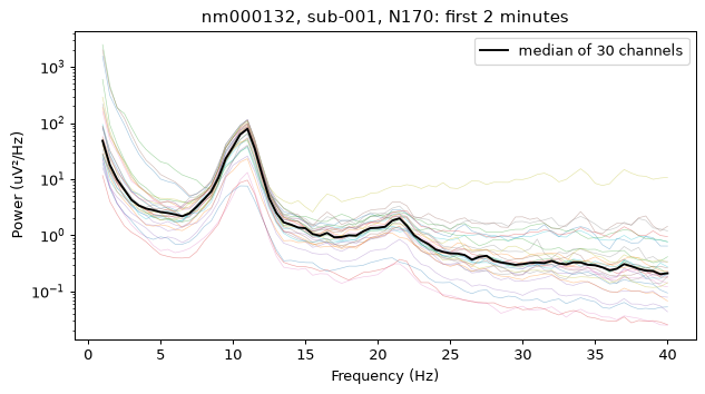

The power spectra of 30 EEG channels from nm000132, subject 001, N170 task, over the first two minutes, on a log scale from 1 to 40 Hz, with their median in black peaking near 11 Hz.

median alpha peak: 11.0 Hz

The median spectrum peaks at 11 Hz, the alpha rhythm, with a smaller peak near 20 Hz.

The events

Each dataset with a Zarr copy has an events.parquet of its events, with each event’s sample_index in the recording. List its columns to see where a dataset names its conditions: ERP CORE’s faces and cars are in event_type.

%pip install pandas fastparquet
import io

import pandas as pd
from pyodide.http import pyfetch

response = await pyfetch("https://zarr.nemar.org/nm000132/zarr/events.parquet")
all_events = pd.read_parquet(io.BytesIO(await response.bytes()), engine="fastparquet")
events = all_events[(all_events.store_path == store.zarr) & (all_events.group_name == group.name)]
print(events.groupby(["trial_type", "event_type"]).size())

trial_type  event_type
response    correct_response      244
            incorrect_response     76
stimulus    car                    80
            face                   80
            scrambled_car          80
            scrambled_face         80
dtype: int64

Agents can get the same events from NEMAR’s Model Context Protocol (MCP) server; see For agents and tools.

The ERP image

An ERP image stacks one channel’s epochs as rows, one panel per condition, with each condition’s average below. This one uses PO8, where the N170 to faces is usually largest. The code re-references to the average of the EEG channels, filters from 0.1 to 30 Hz, cuts epochs from 200 ms before each event to 800 ms after, and drops epochs over 100 µV. It uses names, eeg, np and plt from the power spectrum cell.

from scipy.signal import butter, sosfiltfilt

recording = await eegprep_lean.read_window(
    index, store, group=group, start_sample=0, n_samples=group.n_samples
)
rate = recording.rate
eeg_names = [names[i] for i in eeg]
data = recording.data[eeg].astype(float)
data -= data.mean(axis=0)  # average reference
data = sosfiltfilt(butter(4, [0.1, 30], btype="band", fs=rate, output="sos"), data, axis=1)
po8 = data[eeg_names.index("PO8")]

pre, post = int(0.2 * rate), int(0.8 * rate)  # 200 ms before to 800 ms after
times = np.arange(-pre, post) / rate * 1000


def epochs(condition):
    onsets = events.loc[events.event_type == condition, "sample_index"]
    epoch = np.stack([po8[s - pre : s + post] for s in onsets if s >= pre and s + post <= len(po8)])
    epoch -= epoch[:, :pre].mean(axis=1, keepdims=True)  # baseline
    return epoch[np.abs(epoch).max(axis=1) <= 100]  # drop epochs over 100 uV


faces, scrambled = epochs("face"), epochs("scrambled_face")
smooth = lambda e: np.stack([e[max(0, k - 2) : k + 3].mean(axis=0) for k in range(len(e))])
limit = np.percentile(np.abs(np.concatenate([smooth(faces), smooth(scrambled)])), 98)

fig = plt.figure(figsize=(9, 6.5), layout="constrained")
grid = fig.add_gridspec(2, 2, height_ratios=[3, 1.4])
for col, (title, e) in enumerate([("Faces", faces), ("Scrambled faces", scrambled)]):
    ax = fig.add_subplot(grid[0, col])
    image = ax.imshow(smooth(e), aspect="auto", origin="lower", cmap="RdBu_r",
                      vmin=-limit, vmax=limit, extent=[times[0], times[-1], 0, len(e)])
    ax.axvline(0, color="gray", lw=0.8)
    ax.set(title=f"{title}, PO8 ({len(e)} epochs)", ylabel="Epoch" if col == 0 else None)
fig.colorbar(image, ax=fig.axes, label=recording.unit, shrink=0.8)
average = fig.add_subplot(grid[1, :])
average.plot(times, faces.mean(axis=0), label="faces")
average.plot(times, scrambled.mean(axis=0), label="scrambled faces")
average.plot(times, faces.mean(axis=0) - scrambled.mean(axis=0), color="k", lw=1, label="difference")
average.axvspan(150, 260, color="gray", alpha=0.15)
average.axvline(0, color="gray", lw=0.8)
average.set(xlabel="Time (ms)", ylabel=recording.unit, xlim=(times[0], times[-1]))
average.legend(fontsize=8, loc="upper left")
plt.show()
window = (times >= 150) & (times <= 260)
difference = faces[:, window].mean() - scrambled[:, window].mean()
print(f"150-260 ms at PO8: faces minus scrambled faces {difference:.1f} {recording.unit}")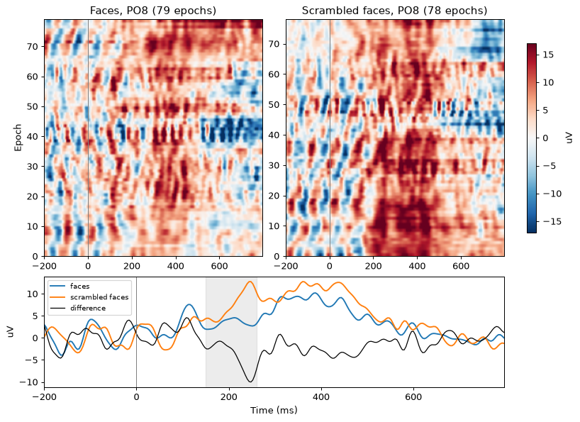

ERP images at PO8 for faces (79 epochs) and scrambled faces (78 epochs) from nm000132, subject 001, and their averages below with the faces minus scrambled faces difference in black, most negative near 250 ms.

150-260 ms at PO8: faces minus scrambled faces -4.3 uV

79 face and 78 scrambled-face epochs pass the 100 µV limit, of 80 each. Faces are more negative than scrambled faces from about 150 ms, most of all near 250 ms, where the difference reaches about -10 µV. That is the face-specific negativity the N170 paradigm measures, later in this subject than the textbook 170 ms. One subject’s ERP from a downsampled copy is a first look; the full analysis belongs on the original files.

Using another dataset

Another recording. [s.path for s in index.stores] lists them; pass one to index.store(...).
Other conditions. Print the events’ columns with their values, as above, and select on the column that names them.
Another channel or unit. Choose the channel the component is known for, and give the rejection limit in the recording’s own unit (recording.unit).
A long recording. Reading one recording whole is cheap here, 33 channels for 11 minutes. For hours of data, read only the channels you need (channels=[...] on read_window), or the span the events cover.